Statistics Canada publishes the Poisson bootstrap for its public use microdata in SAS and R. svy now implements it, and this validates it against the agency’s own reference code.
Labour Force Survey PUMF, Poisson bootstrap, Statistics Canada, survey variance estimation Python, bootstrap weights, replicate weights Python, design-based estimation, complex survey analysis Python, unemployment rate standard error
Summary
TipTL;DR
The Canadian Labour Force Survey public use microdata file (PUMF) ships one weight and no explicit design variables. Therefore, taylor design-based standard errors cannot be computed from it directly. However, Statistics Canada, in section 6 of the PUMF user guide, recommends a Poisson bootstrap method, with reference code in SAS and R provided in the document.
Validated against the agency’s own R code on the July 2026 file, in two parts, because a bootstrap is stochastic and only one of the two halves (i.e. the estimator) can be compared exactly:
Part A — the estimator and the documented formulas. Hand both sides the same Poisson factors and let each build the replicate weights independently. They agree to 7.4e-16 on the estimate and 3.9e-15 on the standard error, across Canada and the ten provinces. That is floating-point round-off.
Part B — svy’s own weight generator. Let svy draw its own factors end to end. The point estimate is identical at every seed, the calibration identity holds to 5e-15, and the standard error sits within Monte Carlo error of the reference.
Everything computed from the PUMF is not seasonally adjusted, and matches Statistics Canada’s published unadjusted series at published precision: 6.7% unemployment, 61.5% employment, 65.9% participation. The Daily’s 6.4% headline is the seasonally adjusted series and is not the right comparison.
Background
The Labour Force Survey is Canada’s monthly household labour market survey and the source of the national unemployment rate. Its public use file carries 113,603 records for July 2026 across 60 variables.
ImportantEvery estimate here is unadjusted for seasonality
The PUMF carries no seasonal adjustment, so everything computed from it is a not seasonally adjusted estimate. Statistics Canada publishes both series, and they answer different questions:
Seasonally adjusted (The Daily and table 14-10-0287). This is the 6.4% headline for July 2026, and it is the series to use for month-over-month comparisons.
Unadjusted (table 14-10-0017). This is what the PUMF reproduces: 6.7% for July 2026.
Sixty variables, and exactly one is a weight: FINALWT. No stratum identifier, no primary sampling unit, no replicate weights. The user guide says why:
The calculation of precise variance estimates requires detailed knowledge of the sample design of the survey. To protect the confidentiality of respondents, this level of detail cannot be included in a PUMF.
The LFS runs a six-month rotating panel with composite estimation on top of calibration to population projections. For confidentiality reasons, Statistics Canada does not include the design variables in the PUMF. However, they prescribed the Poisson bootstrap for variance estimation including the recommended calibration domains and detailled SAS and R code examples.
What Statistics Canada publishes
For public users the agency documents a substitute: a Poisson bootstrap, citing Beaumont and Patak (2012), described as a special case of the generalized bootstrap.
The specification is complete. Equation numbers below are the guide’s own, so they can be checked against section 6.1 of the PDF directly. For each unit \(k\):
where \(poissonfactor_k\) is \(+1\) or \(-1\) with probability one half, drawn independently for every unit and every replicate, repeated to build 1,000 replicates. The uncalibrated bootstrap weight is then
\[bootwt_k = \alpha_k \times finalwt_k \tag{2}\]
Statistics Canada mentioned that a calibrated version of the Poisson bootstrap can lead to variance estimates that are closer to those estimated by the LFS master file. Calibration is done by adjusting each of the uncalibrated bootstrap weights using:
where \(g\) indicates the calibration domain. In the case of the LFS survey, the domain are chosen to be similar to those used in the calibration of the master data file: province, age group, and gender.
Appendix D ships reference code in SAS and R. There was no Python implementation, which is what svy now closes.
NoteWhy independent draws are the point
Rao-Wu replicate weights encode stratum and PSU structure, which is exactly why they cannot be published. Poisson bootstrap weights are drawn independently per unit, so they carry no design information and are safe to release.
Using it
The whole workflow is three calls. where restricts to the labour force without subsetting the design, and by estimates across all ten provinces in one pass:
View code
domains = ["PROV", "GENDER", "age_cal"]controls = {tuple(r[c] for c in domains): r["total"]for r in pumf.group_by(domains).agg(pl.col("FINALWT").sum().alias("total")).to_dicts()}sample = ( svy.Sample(data=pumf, design=svy.Design(wgt="FINALWT")) .weighting.create_bs_wgts(n_reps=1000, kind="poisson") .weighting.poststratify(controls=controls, by=domains))by_province = sample.estimation.prop("unemployed", method="replication", where=~pl.col("nilf"), variance_center="estimate", by="PROV",)
The two steps are deliberately separate. Equations (1) and (2) are the bootstrap, and the guide ends them at “Repeat this procedure to create 1,000 bootstrap replicates”; calibration arrives afterwards as “a calibrated version” that “can” bring the variance closer to a master-file estimate. It is ordinary post-stratification, it applies to any replicate method rather than this one, and poststratify adjusts the replicate columns alongside the main weight unless ignore_reps=True. Skip it and you have the uncalibrated bootstrap, which is a different estimator. As with everything computed from the PUMF, the resulting estimates are not seasonally adjusted.
The design records which algorithm produced the weights, so a reader can tell afterwards:
Validating a stochastic estimator across languages
A bootstrap draws random numbers, so svy and R cannot produce identical weights: their generators differ, and demanding bit-equality would be testing the seed rather than the method. The comparison splits in two.
Part A — the estimators, on identical weights
The Poisson factors are drawn once and shared, and each side builds its own replicate weights from them using equations (1), (2) and (3): NumPy on the Python side, and on the R side Appendix D2 unchanged apart from reading the factor file instead of calling sample(). The two weight matrices come out bit-identical — 11.4 million values, zero difference — so the weights are not a variable here and anything that differs downstream is the estimator alone.
svy then takes those weights as an ordinary replication design. Its own generator is not involved; that is Part B.
July 2026 unemployment rate, not seasonally adjusted, labour force aged 15 and over, 1,000 calibrated replicates:
Rate
svy SE
StatCan SE
Relative difference
Canada
6.6806%
0.12357%
0.12357%
3.9e-15
Newfoundland and Labrador
8.0509%
0.46667%
0.46667%
5.6e-16
Prince Edward Island
6.4371%
0.56353%
0.56353%
6.2e-16
Nova Scotia
6.5032%
0.41322%
0.41322%
6.3e-16
New Brunswick
6.8708%
0.39735%
0.39735%
2.2e-16
Quebec
5.6161%
0.29841%
0.29841%
2.2e-15
Ontario
7.2830%
0.19814%
0.19814%
6.6e-16
Manitoba
5.4606%
0.37477%
0.37477%
4.6e-16
Saskatchewan
6.3744%
0.37121%
0.37121%
7.0e-16
Alberta
7.1185%
0.44318%
0.44318%
7.8e-16
British Columbia
6.4825%
0.31567%
0.31567%
5.5e-16
Maximum relative difference across all eleven domains: 7.4e-16 on the point estimate, 3.9e-15 on the standard error. Double precision carries roughly 16 significant digits, so this is round-off, not agreement to a tolerance.
Part B — svy generating the weights end to end
Now svy does the whole thing: create_bs_wgts(kind="poisson") draws its own Poisson factors in Rust and builds the replicate weights, and poststratify calibrates them. This is the only place svy’s generator runs, and it is why the comparison here cannot be exact — svy’s factors are not R’s, and demanding bit-equality across two languages’ generators would be testing the seed rather than the method.
Three properties are checkable without a shared draw.
The point estimate does not depend on the seed. It is computed from FINALWT alone; the replicates only inform the variance. Across eight seeds it is 6.6806% every time, bit-identical.
The calibration identity holds exactly. Every replicate reproduces the FINALWT total within each province × gender × age domain, to a maximum relative deviation of 5.2e-15. All replicate weights are strictly positive, as the method guarantees.
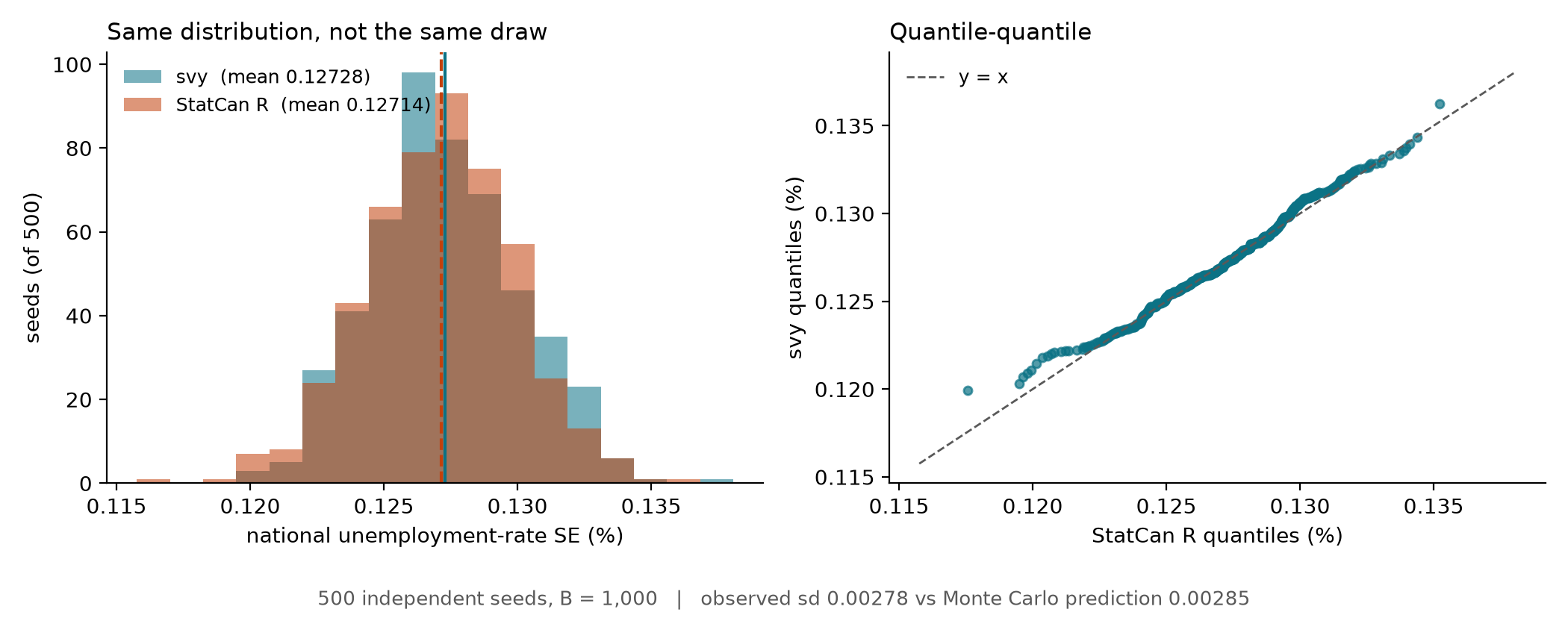
The standard error is a random variable, so compare distributions. Running both engines over 500 independent seeds at B = 1,000 gives two samples of the national SE that can be compared directly.
Figure 1: svy and Statistics Canada’s Appendix D2, each run 500 times with its own random draw. Left: the two distributions of the national unemployment-rate standard error. Right: their quantiles against each other.
They agree on the mean to 0.12728% against 0.12714%, and on the spread to 0.00278% against 0.00280%. The difference of means is +0.000147 with a 95% interval of [-0.000199, +0.000493], so any systematic difference between the generators is under 0.4% of the standard error itself. A Kolmogorov-Smirnov test does not separate the two samples (p = 0.51).
The bound is the useful number there, not the p-value: failing to reject tells you nothing, whereas a tight interval around zero says how large a difference the data would have caught.
What is left is Monte Carlo noise, and it is the right size. At B replicates the sampling error of a bootstrap standard error is about \(\mathrm{SE}/\sqrt{2B}\), which is 0.00285% here — against an observed spread of 0.00278%. The scatter between the two engines is therefore what the arithmetic of resampling predicts, with no room left for an implementation difference to hide in. The single draw used in Part A gave 0.12357%, 1.3 standard deviations below the mean: an ordinary seed.
This is also why an exact comparison would be the wrong test. Two correct implementations differ in the third significant figure as a matter of course, so demanding four-figure agreement between independent draws would measure noise and report it as a bug.
NoteWhat each part covers
checked against
how
the estimator, given weights
StatCan’s Appendix D2
exact, 4e-15
equations (1)–(3)
StatCan’s Appendix D2
exact, via the shared factor matrix
svy’s weight generator
the guide’s formulas (1)+(2)
exact, to 1 ULP
svy’s weight generator
StatCan’s Appendix D2
distributional, 500 seeds, difference bounded under 0.4%
The last row is weaker than the others by construction: two generators cannot be compared draw by draw. It is bounded rather than exact.
centring on the full-sample estimate. There is no option for it in Appendix D2 — bs_var <- mean((est_bs - est_fw)^2) is written once, in both bs_total and bs_ratio.
svy defaults to centring on the mean of the replicates instead. The two differ by exactly the squared bootstrap bias \((\bar\theta_b - \hat\theta)^2\), so the agency’s convention is never the smaller of the two, and matching it is one argument:
How much it matters depends entirely on \(B\), and not only in size. At B = 1,000 the national standard error moves by 0.03%. At B = 10 the difference is not merely larger but erratic: across twenty disjoint draws from the same file it ranged from 0.000% to 68.9%, because the bootstrap bias is itself a noisy quantity when there are ten replicates to estimate it from. That is a reason to use a production replicate count rather than a reason to prefer one centring — neither is wrong, but they are not interchangeable, and reproducing a producer’s published variance means matching theirs.
On the published figure
The rate above is 6.68%, not seasonally adjusted. The Daily reported 6.4% for July 2026, and the two are not in conflict: that release states that “unless otherwise stated, estimates presented in this release are seasonally adjusted,” while the PUMF carries no seasonal adjustment at all.
Statistics Canada also publishes the unadjusted series, in table 14-10-0017. Against those figures the PUMF reproduces every headline rate at published precision:
July 2026, unadjusted
From the PUMF
Published
Unemployment rate
6.68%
6.7%
Employment rate
61.51%
61.5%
Participation rate
65.91%
65.9%
The levels agree too, to within a couple of hundred people in a population of 34.8 million:
Level (thousands)
From the PUMF
Published
Difference
Population 15+
34,812.1
34,812.1
5 persons
Labour force
22,944.9
22,945.1
154 persons
Employment
21,412.1
21,412.3
205 persons
Unemployment
1,532.9
1,532.9
49 persons
The largest gap is 0.0006% of the population, which is the confidentiality modification the guide warns about rather than anything to reconcile. The guide is explicit about precedence:
In the case of a discrepancy, estimates in published tables and other data products on the Statistics Canada website should be considered official statistics.
So nothing here audits the official number. But it is worth knowing that the public file, used as documented, lands on the published unadjusted estimates and that comparing it against the seasonally adjusted headline instead would manufacture a 0.28 point discrepancy out of nothing.
References
Beaumont, J.-F. and Patak, Z. (2012). On the generalized bootstrap for sample surveys with special attention to Poisson sampling. International Statistical Review, 80(1), 127-148.
Statistics Canada (2025). Labour Force Survey Public Use Microdata File User Guide. Catalogue 71M0001X.
Statistics Canada (2017). Methodology of the Canadian Labour Force Survey. Catalogue 71-526-X.
Adapted from Statistics Canada, Labour Force Survey Public Use Microdata File, July 2026. This does not constitute an endorsement by Statistics Canada of this product.
TipCommunity signal
Help make svy the standard for survey analysis in Python
If rigorous, design-based survey inference in Python matters to you, starring the repository helps signal demand and prioritize validation and stability work.