Checking a Fay–Herriot Model in Python with svy-sae

Findings, model tests, influence, plots, and calibration

Tutorials

Area-level

Diagnostics

Python

Check a Fay-Herriot small area model in Python with svy-sae: findings with codes, normality and goodness-of-fit tests, Cook’s distance, diagnostic plots, and calibration against higher-level estimates.

Author

Mamadou S. Diallo, Ph.D.

Modified

November 5, 2026

Keywords

Fay-Herriot diagnostics, small area model checking Python, Cook’s distance small areas, Brown goodness-of-fit test, SAE diagnostic plots, calibration small area estimates

About these examples

This tutorial illustrates the svy-sae API; it is not a rigorous small area analysis. The models are kept simple so each step stays readable, and in many places, from the choice of covariates to the variance model, better choices could be made to improve them.

The Fay–Herriot model rests on assumptions: normal area effects and sampling errors, a linear relation with the covariates, and sampling variances that are right. Its estimates are only as good as those assumptions, so check them before publishing.

Every fh() fit computes its checks when it is fitted and stores them with the results, so they need no access to the data afterwards. Rules applied to those checks produce findings, each with a code, in the same form as svy’s warnings.

This tutorial demonstrates how to read the findings, the model-level tests, and the per-district diagnostics, find influential districts, draw the diagnostic plots, and compare the estimates with regional estimates.

Not a search for the best model

This tutorial does not try to find the best model for these data. It shows the options svy-sae offers to evaluate a model and the ways to improve it; the choices made below are examples, not recommendations.

Setting up the inputs

We continue with the inputs from the previous tutorials, and fit the model chosen in Choosing covariates next to the baseline without covariates:

Rebuild the inputs from Preparing inputs

import polars as pl
import svy

import svy_sae as sae

hld_data = svy.datasets.load("hld_sample_wb_2023").data
hld_design = svy.Design(stratum=("geo1", "urbrur"), psu="ea", wgt="hhweight")
hld_sample = svy.Sample(data=hld_data, design=hld_design).wrangling.mutate(
    {
        "hhpovline": svy.col("hhsize") * 1800,
        "pov_status": svy.when(svy.col("tot_exp") < svy.col("hhpovline")).then(1).otherwise(0),
    }
)

direct = (
    hld_sample.estimation.prop(y="pov_status", by="geo2")
    .to_polars()
    .filter(pl.col("pov_status") == 1)
    .select("geo2", "est", "se", "cv", "lci", "uci", "df", "n")
    .with_columns((pl.col("se") ** 2).alias("var_direct"))
)

hld_census = svy.datasets.load("hld_pop_wb_2023").data
yes_no = ["electricity", "car", "refrigerator", "tv", "cell", "bank"]
district_x = (
    hld_census.group_by("geo1", "geo2")
    .agg(
        (pl.col("urbrur") == "Urban").mean().alias("urban"),
        (pl.col("piped_water") != "No piped water").mean().alias("piped_water"),
        (pl.col("flush_toilet") == "Flush toilet").mean().alias("flush_toilet"),
        *[(pl.col(c) == "Yes").mean().alias(c) for c in yes_no],
        pl.col("hhsize").mean().alias("hhsize"),
        pl.col("rooms").mean().alias("rooms"),
        pl.len().alias("n_hh"),
    )
    .sort("geo2")
)

truth = (
    hld_census.group_by("geo2")
    .agg((pl.col("tot_exp") < pl.col("hhsize") * 1800).mean().alias("true_rate"))
    .sort("geo2")
)

direct = direct.with_columns(pl.col("n").log().alias("log_n"))
smoothed = sae.smooth_variance(direct, x="log_n", variance="var_direct", df="df")
model = sae.AreaLevel(smoothed)

fit_base = model.fh(
    y="est", x=[], area="geo2", variance="variance_smoothed", pop_data=district_x
)
fit = model.fh(
    y="est", x=["piped_water"], area="geo2", variance="variance_smoothed", pop_data=district_x
)

Findings

The findings are printed at the bottom of the results, and exported with to_polars("findings"):

fit.to_polars("findings").select("code", "level", "title", "detail")

shape: (3, 4)

code	level	title	detail
str	str	str	str
"SAE_SIGMA_U_BOUNDARY"	"warning"	"Area variance at the boundary"	"sigma_u^2 is 4.2e-05 of the me…
"SAE_INFLUENTIAL_AREAS"	"warning"	"2 influential areas"	"Cook's distance above 0.0678: …
"SAE_HIGH_CV"	"info"	"12 of 61 areas with CV above 0…	"Areas: ['geo_01_01', 'geo_01_0…

Each has a level (warning or info), a title, the detail behind it, and often a hint. The rules and their codes:

Table 1: Findings of a Fay–Herriot fit

Code	Raised when
`SAE_SIGMA_U_BOUNDARY`	\(\hat\sigma^2_u\) is below `boundary_tol` times the median sampling variance
`SAE_NONNORMAL_RESIDUALS`	Shapiro–Wilk rejects normality of the standardized residuals at `alpha`
`SAE_NONNORMAL_AREA_EFFECTS`	Shapiro–Wilk rejects normality of the standardized area effects at `alpha`
`SAE_INFLUENTIAL_AREAS`	An area’s Cook’s distance exceeds `cooks_max` (default \(4/m\) for \(m\) sampled areas)
`SAE_BIAS_VS_DIRECT`	The Brown test rejects agreement between model and direct estimates at `alpha`
`SAE_RESIDUAL_PATTERN`	Residuals correlate with the synthetic estimate or a covariate at `alpha`
`SAE_COLLINEARITY`	A covariate’s variance inflation factor exceeds `vif_max`
`SAE_HIGH_CV`	An estimate’s CV exceeds `cv_max`
`SAE_NO_CV_GAIN`	A sampled area’s model CV is not below its direct CV
`SAE_BENCHMARK_LARGE`	Benchmarking moved a group by more than `shift_max`

The model with piped water raises three. The boundary was explained in The Fay–Herriot model: the covariate leaves almost no variation between districts. The influential districts are examined below. The high CVs are an info: most districts are now well below 30%.

The baseline raises more:

fit_base.to_polars("findings").select("code", "title")

shape: (5, 2)

code	title
str	str
"SAE_NONNORMAL_RESIDUALS"	"Residuals not normal"
"SAE_NONNORMAL_AREA_EFFECTS"	"Area effects not normal"
"SAE_INFLUENTIAL_AREAS"	"2 influential areas"
"SAE_HIGH_CV"	"41 of 61 areas with CV above 0…
"SAE_NO_CV_GAIN"	"6 sampled areas without a prec…

Without covariates, the residuals and area effects are not normal, and six districts gain no precision from the model.

Changing the thresholds

diagnostics.findings() applies the rules again with other thresholds:

[(f.code, f.title) for f in fit.diagnostics.findings(cv_max=0.2, boundary_tol=1e-6)]

[('SAE_INFLUENTIAL_AREAS', '2 influential areas'),
 ('SAE_HIGH_CV', '19 of 61 areas with CV above 0.2')]

Its arguments are alpha (0.05), cv_max (0.3), boundary_tol (0.001), cooks_max (\(4/m\)), shift_max (0.1), and vif_max (10). They change only the rules, never the stored statistics.

Model-level tests

The statistics behind the findings:

fit.to_polars("tests")

shape: (14, 5)

name	applies_to	statistic	df	p_value
str	str	f64	f64	f64
"shapiro_residuals"	"residuals"	0.981229	null	0.49425
"skewness_residuals"	"residuals"	0.117548	null	null
"kurtosis_residuals"	"residuals"	3.339098	null	null
"shapiro_area_effects"	"area_effects"	0.977658	null	0.348468
"skewness_area_effects"	"area_effects"	0.510638	null	null
…	…	…	…	…
"synthetic_direct_correlation"	"model"	0.512491	null	null
"sigma_u2_to_median_d"	"model"	0.000042	null	null
"resid_vs_synthetic"	"residuals"	-0.07876	null	0.55322
"resid_vs_piped_water"	"residuals"	0.07876	null	0.55322
"vif_piped_water"	"covariates"	1.0	null	null

Table 2: Model-level tests

Test	What it measures
`shapiro_`, `skewness_`, `kurtosis_*`	Normality of the standardized residuals and area effects
`adj_r2`, `fh_r2`	Share of the variation explained by the covariates; `fh_r2` accounts for the sampling variances
`brown`	Goodness of fit of the model estimates to the direct ones, a chi-square on \(m\) degrees of freedom
`synthetic_direct_correlation`	Correlation of the synthetic and direct estimates
`sigma_u2_to_median_d`	\(\hat\sigma^2_u\) relative to the median sampling variance
`resid_vs_*`	Correlation of the residuals with the synthetic estimate and each covariate
`vif_*`	Variance inflation factor of each covariate

Look one up by name:

print(fit.diagnostics.test("brown"))

DiagTest(name='brown', applies_to='model', statistic=62.920941576116434, df=59.0, p_value=0.3393120249726548, indicator=None, time=None)

The Brown test does not reject: the model estimates are consistent with the direct ones given their sampling variances.

Per-district diagnostics

One row per district, including those outside the sample:

diagnostics = fit.to_polars("diagnostics")

diagnostics.columns

['area',
 'in_sample',
 'pred',
 'mse',
 'cv',
 'direct',
 'direct_var',
 'direct_cv',
 'synthetic',
 'fitted',
 'gamma',
 'u_hat',
 'u_std',
 'resid_std',
 'cooks_d',
 'x_piped_water']

Next to the estimate and its MSE and CV, the table has the direct estimate and its variance and CV, the synthetic estimate and the fitted value, the shrinkage factor gamma, the area effect u_hat and its standardized value u_std, the standardized residual resid_std, Cook’s distance cooks_d, and each covariate as x_<name>.

Influential districts

Cook’s distance measures how much the fitted coefficients move when a district is left out. Sort by it:

diagnostics.sort("cooks_d", descending=True, nulls_last=True).select(
    "area", "direct", "direct_var", "synthetic", "pred", "resid_std", "cooks_d"
).head(4)

shape: (4, 7)

area	direct	direct_var	synthetic	pred	resid_std	cooks_d
str	f64	f64	f64	f64	f64	f64
"geo_05_03"	0.69343	0.013836	0.35818	0.358194	2.850039	0.158798
"geo_05_01"	0.055238	0.024909	0.393654	0.393646	-2.144171	0.068034
"geo_09_02"	0.535227	0.01145	0.341294	0.341303	1.812317	0.065946
"geo_10_01"	0.0	0.024909	0.362384	0.362376	-2.296035	0.057743

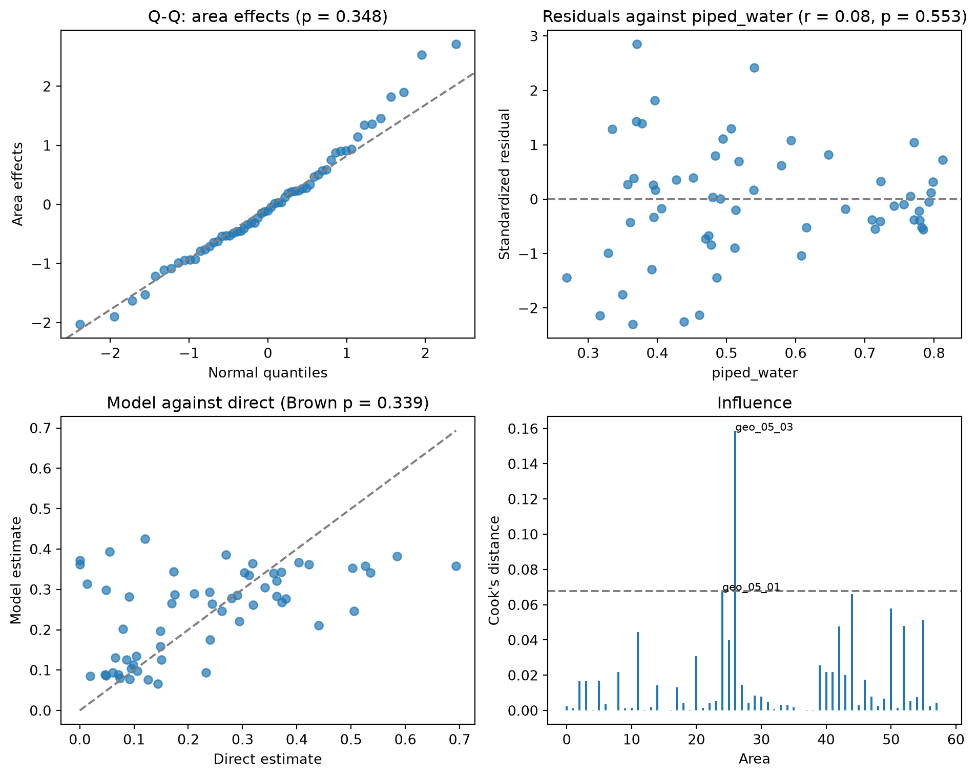
geo_05_03 has a direct poverty rate of 69%, against a synthetic 36%; geo_05_01 has 6% against 39%. Refit without them and see how far the estimates move:

influential = ["geo_05_01", "geo_05_03"]
fit_without = sae.AreaLevel(smoothed.filter(~pl.col("geo2").is_in(influential))).fh(
    y="est", x=["piped_water"], area="geo2", variance="variance_smoothed", pop_data=district_x
)

shift = (
    fit.to_polars("predictions").select("area", "pred")
    .join(fit_without.to_polars("predictions").select("area", pl.col("pred").alias("without")), on="area")
    .select(pl.col("area"), (pl.col("without") - pl.col("pred")).abs().alias("shift"))
)

print(f"Largest change in any estimate: {shift['shift'].max():.4f}")

Largest change in any estimate: 0.0057

The two districts still get estimates, from the census covariates, and no estimate moves by more than a percentage point. They are influential by Cook’s rule of thumb, but they do not drive the results.

Diagnostic plots

fit.plots draws from the stored diagnostics. Each plot takes ax= and returns the matplotlib axes, so plots combine into figures. The plots need matplotlib: pip install "svy-sae[plot]".

import matplotlib.pyplot as plt

fig, axes = plt.subplots(2, 2, figsize=(10, 8))
fit.plots.qq(ax=axes[0, 0])
fit.plots.residuals(against="piped_water", ax=axes[0, 1])
fit.plots.model_vs_direct(ax=axes[1, 0])
fit.plots.cooks(ax=axes[1, 1])
fig.tight_layout()

Diagnostic plots for the model with piped water

Table 3: Diagnostic plots

Plot	Shows
`qq(level="area")`	Normal Q-Q plot of the standardized area effects (`level="residual"` for the residuals)
`residuals(against="fitted")`	Standardized residuals against the fitted values or a covariate
`shrinkage()`	Weight on the direct estimate against the sampling variance
`model_vs_direct()`	Model estimates against direct estimates, with the 45-degree line
`cv()`	CVs of the direct and model estimates, districts ordered by direct CV
`cooks(threshold=None)`	Cook’s distance by district, with the threshold
`benchmark()`	Change made to each group by benchmarking
`compare(*others, what="cv")`	This fit against other fits, by CV or by estimate

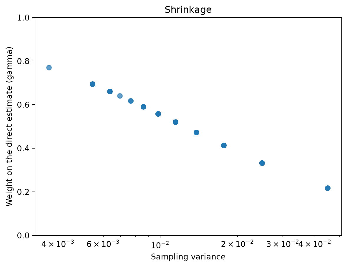
With the area variance at the boundary, every gamma is near zero and the shrinkage plot is flat. The baseline shows what it looks like when the model shrinks: the noisier a district’s direct estimate, the less weight it keeps:

fit_base.plots.shrinkage();

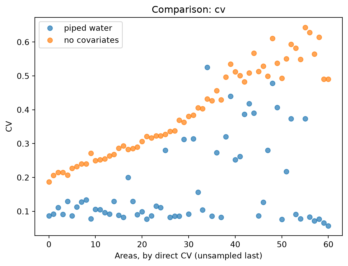
compare() puts fits side by side. Piped water lowers the CV of almost every district:

fit.plots.compare(fit_base, labels=["piped water", "no covariates"]);

Calibration against regional estimates

The survey supports reliable estimates for the ten regions. diagnostics.calibration() aggregates the district estimates to regions, weighting by the number of households, and compares them with targets, adjusting nothing:

regional = (
    hld_sample.estimation.prop(y="pov_status", by="geo1")
    .to_polars()
    .filter(pl.col("pov_status") == 1)
    .select("geo1", pl.col("est").alias("target"), "se")
)

calibration = fit.diagnostics.calibration(
    targets=regional, sizes=district_x, area="geo2", size="n_hh", group="geo1"
)

calibration

shape: (10, 4)

geo1	target	aggregate	difference
str	f64	f64	f64
"geo_01"	0.085854	0.084013	-0.021451
"geo_02"	0.341601	0.327366	-0.041672
"geo_03"	0.218635	0.193967	-0.112827
"geo_04"	0.171531	0.17307	0.008973
"geo_05"	0.323229	0.307004	-0.050197
"geo_06"	0.218746	0.26723	0.221648
"geo_07"	0.227652	0.235576	0.034809
"geo_08"	0.252795	0.348402	0.378198
"geo_09"	0.320075	0.268993	-0.159595
"geo_10"	0.227131	0.23195	0.021217

difference is the aggregate over the target, minus one. Some regions are far apart. But a regional direct estimate is an estimate too, with its own error. Add the regional standard errors and the true regional rates:

regional_truth = hld_census.group_by("geo1").agg(
    (pl.col("tot_exp") < pl.col("hhsize") * 1800).mean().alias("true_rate")
)

calibration.join(regional, on=["geo1", "target"]).join(regional_truth, on="geo1").select(
    "geo1", "target", "se", "aggregate", "true_rate"
).sort("geo1")

shape: (10, 5)

geo1	target	se	aggregate	true_rate
str	f64	f64	f64	f64
"geo_01"	0.085854	0.018468	0.084013	0.101067
"geo_02"	0.341601	0.057104	0.327366	0.362653
"geo_03"	0.218635	0.037784	0.193967	0.225458
"geo_04"	0.171531	0.035423	0.17307	0.188191
"geo_05"	0.323229	0.061502	0.307004	0.319634
"geo_06"	0.218746	0.051654	0.26723	0.284173
"geo_07"	0.227652	0.051374	0.235576	0.266986
"geo_08"	0.252795	0.082375	0.348402	0.347916
"geo_09"	0.320075	0.044651	0.268993	0.288468
"geo_10"	0.227131	0.036828	0.23195	0.256449

In geo_08, the largest gap, the model’s aggregate matches the true rate. The regional direct estimate is the one that is off, by about one of its standard errors: ordinary sampling error. A gap between model and direct estimates is a question to look into, not proof that the model is wrong. Benchmarking forces the two to agree, so check calibration before deciding to benchmark.

Summary

This tutorial checked the Fay–Herriot model:

Findings with codes, from to_polars("findings"), re-applied with other thresholds by diagnostics.findings()
Model-level tests in to_polars("tests"): normality, R², the Brown test, residual correlations, and VIFs
Per-district diagnostics in to_polars("diagnostics"), and influential districts by Cook’s distance, checked by refitting without them
Plots from fit.plots, each on its own axes
Calibration of the aggregated estimates against regional estimates, which have errors of their own

Next steps

Poverty rates are proportions, bounded by 0 and 1. A transformation keeps the model on a scale where that bound holds.

Transform the outcome
Continue to Transformations →