Checking Unit-Level Models in Python with svy-sae

Unit and district diagnostics, findings, and plots

Check unit-level small area models in Python with svy-sae: residuals and Cook’s distance for every sampled unit and area, normality, R² and ICC, findings, diagnostic plots, and what a transformation changes.

Keywords

unit-level model diagnostics, nested error regression diagnostics, Cook’s distance mixed model, ICC small area estimation, EBLUP EBP model checking Python

WarningAbout these examples

This tutorial illustrates the svy-sae API; it is not a rigorous small area analysis. The models are kept simple so each step stays readable, and in many places, from the choice of covariates to the variance model, better choices could be made to improve them.

The BHF model assumes that the area effects and the unit errors are normal, and that the outcome is linear in the covariates. The BHF model found its MSE well below the actual error of its estimates, a sign that these assumptions fail.

Every eblup() and ebp() fit computes its checks when it is fitted: one row per sampled unit, one row per area, and model-level tests, with findings from rules on them, as at the area level.

This tutorial demonstrates how to read the unit-level findings, tests, and tables, trace an influential household back to the data, draw the diagnostic plots, and see what a transformation changes.

NoteNot a search for the best model

This tutorial does not try to find the best model for these data. It shows the options svy-sae offers to evaluate a model and the ways to improve it; the choices made below are examples, not recommendations.

Setting up the inputs

We continue with the inputs and the model of The BHF model:

import polars as pl
import svy

import svy_sae as sae

yes_no = ["electricity", "car", "refrigerator", "tv", "cell", "bank"]
covariates = [
    "urban", "piped_water", "flush_toilet", *yes_no, "hhsize", "rooms",
]


def household_covariates(frame):
    return frame.with_columns(
        (pl.col("tot_exp") / pl.col("hhsize")).alias("exp_pp"),
        (pl.col("urbrur") == "Urban").cast(pl.Float64).alias("urban"),
        (pl.col("piped_water") != "No piped water").cast(pl.Float64).alias("piped_water"),
        (pl.col("flush_toilet") == "Flush toilet").cast(pl.Float64).alias("flush_toilet"),
        *[(pl.col(c) == "Yes").cast(pl.Float64).alias(c) for c in yes_no],
        pl.col("hhsize").cast(pl.Float64),
        pl.col("rooms").cast(pl.Float64),
    )


hld_data = household_covariates(svy.datasets.load("hld_sample_wb_2023").data)
hld_census = household_covariates(svy.datasets.load("hld_pop_wb_2023").data)

census_units = hld_census.select("geo1", "geo2", *covariates)
census_means = hld_census.group_by("geo2").agg(
    *[pl.col(c).mean() for c in covariates], pl.len().alias("n_hh")
)

truth = hld_census.group_by("geo2").agg(
    pl.col("exp_pp").mean().alias("true_mean"),
    (pl.col("exp_pp") < 1800).mean().alias("true_rate"),
)

model = sae.UnitLevel(hld_data)

fit = model.eblup(
    y="exp_pp", x=covariates, area="geo2", pop_data=census_means, pop_size="n_hh"
)

Findings

fit.to_polars("findings").select("code", "title", "detail")

shape: (2, 3)

code	title	detail
str	str	str
"SAE_NONNORMAL_AREA_EFFECTS"	"Area effects not normal"	"Shapiro-Wilk W = 0.923, p = 0.…
"SAE_INFLUENTIAL_AREAS"	"19 influential areas"	"Cook's distance above 0.0678: …

Unit-level fits apply a subset of the area-level rules, with the same codes:

Table 1: Findings of a unit-level fit

Code	Raised when
SAE_SIGMA_U_BOUNDARY	The intra-area correlation (ICC) is below boundary_tol
SAE_NONNORMAL_RESIDUALS	Shapiro–Wilk rejects normality of the unit residuals at alpha
SAE_NONNORMAL_AREA_EFFECTS	Shapiro–Wilk rejects normality of the predicted area effects at alpha
SAE_INFLUENTIAL_AREAS	An area’s Cook’s distance exceeds cooks_max (default \(4/m\) for \(m\) sampled areas)
SAE_COLLINEARITY	A covariate’s variance inflation factor exceeds vif_max

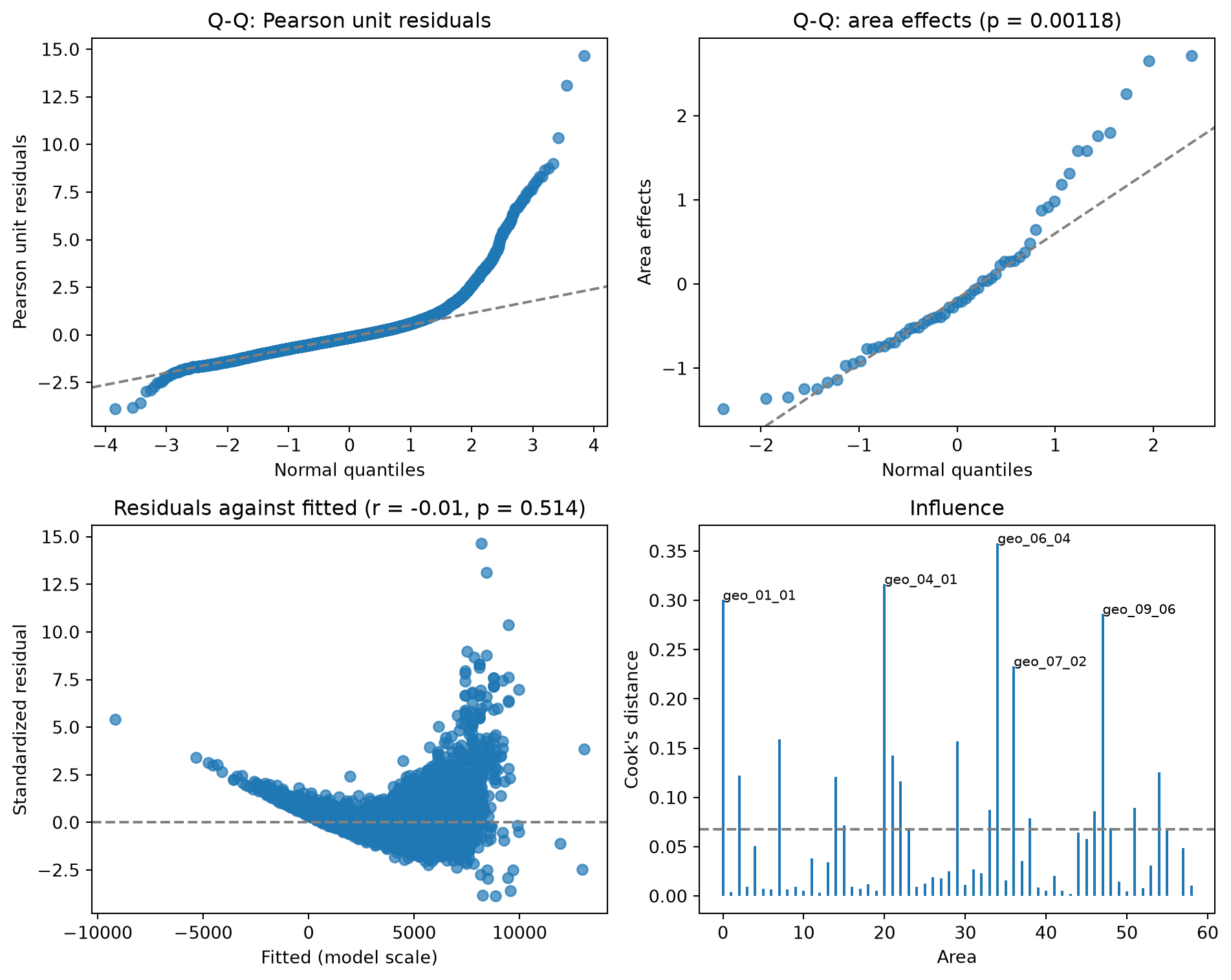
The area effects are not normal, and many districts are influential by the default rule. There is no finding on the unit residuals, but not because they are normal.

Model-level tests

fit.to_polars("tests").filter(
    ~pl.col("name").str.starts_with("resid_vs_") & ~pl.col("name").str.starts_with("vif_")
)

shape: (8, 5)

name	applies_to	statistic	df	p_value
str	str	f64	f64	f64
"skewness_residuals"	"residuals"	3.292844	null	null
"kurtosis_residuals"	"residuals"	26.214082	null	null
"shapiro_area_effects"	"area_effects"	0.92347	null	0.00118
"skewness_area_effects"	"area_effects"	0.955485	null	null
"kurtosis_area_effects"	"area_effects"	3.405518	null	null
"r2_marginal"	"model"	0.580099	null	null
"r2_conditional"	"model"	0.59805	null	null
"icc"	"model"	0.042753	null	null

Table 2: Unit-level model tests

Test	What it measures
shapiro_*, skewness_*, kurtosis_*	Normality of the Pearson unit residuals and of the predicted area effects
r2_marginal	Share of the variance explained by the covariates
r2_conditional	Share explained by the covariates and the area effects
icc	Intra-area correlation, \(\sigma^2_u / (\sigma^2_u + \sigma^2_e)\)
resid_vs_*	Correlation of the residuals with the fitted values and each covariate
vif_*	Variance inflation factor of each covariate
boxcox_lambda, boxcox_shift	For Box–Cox EBP fits, the transformation used

The unit residuals have a skewness of 3.3 and a kurtosis of 26, against 0 and 3 for a normal distribution: expenditure has a long right tail that the model does not capture.

WarningNo normality test past 5,000 units

Shapiro–Wilk is computed for 3 to 5,000 values, as in R’s shapiro.test. With more sampled units, as here, there is no shapiro_residuals test and no SAE_NONNORMAL_RESIDUALS finding: read the skewness and kurtosis, and the Q-Q plot below.

The covariates explain most of the variation (r2_marginal), and the area effects add little to it: the ICC says that 4% of the remaining variance lies between districts.

Unit diagnostics

One row per sampled household:

units = fit.to_polars("units")

units.columns

['row',
 'area',
 'y',
 'fitted_marginal',
 'fitted_conditional',
 'resid_marginal',
 'resid_conditional',
 'resid_pearson',
 'cooks_d',
 'x_urban',
 'x_piped_water',
 'x_flush_toilet',
 'x_electricity',
 'x_car',
 'x_refrigerator',
 'x_tv',
 'x_cell',
 'x_bank',
 'x_hhsize',
 'x_rooms']

Table 3: Unit diagnostics

Column	Content
row	Position of the unit in the data passed to UnitLevel
area, y	Area and outcome
fitted_marginal, fitted_conditional	\(x'\hat\beta\), and \(x'\hat\beta + \hat u_i\)
resid_marginal, resid_conditional	The outcome minus each fitted value
resid_pearson	Residual scaled by \(\hat\sigma_e\)
cooks_d	Cook’s distance for deleting the unit
x_<name>	Each covariate

The households with the largest Cook’s distance:

units.sort("cooks_d", descending=True).select(
    "row", "area", "y", "fitted_conditional", "resid_pearson", "cooks_d"
).head()

shape: (5, 6)

row	area	y	fitted_conditional	resid_pearson	cooks_d
i64	str	f64	f64	f64	f64
3862	"geo_04_04"	20046.5	12577.652086	3.837463	0.025867
5200	"geo_06_04"	3021.5	10363.214278	-3.593227	0.025733
7589	"geo_10_06"	1269.666667	8108.341617	-3.829714	0.024572
7179	"geo_10_02"	1796.0	8593.847153	-3.866803	0.02452
6241	"geo_09_02"	707.727273	-8221.001663	5.411056	0.018174

One of them has a negative fitted expenditure. row finds the households with one in the data:

negative = units.filter(pl.col("fitted_conditional") < 0)["row"].to_list()

flagged = hld_data.with_row_index("row").filter(pl.col("row").is_in(negative))

print(f"Households with a negative fitted value: {flagged.height}")
print(f"Their median size: {flagged['hhsize'].median():.0f}, against {hld_data['hhsize'].median():.0f} overall")

Households with a negative fitted value: 314
Their median size: 8, against 4 overall

They are large households. Each member lowers the fitted value by the hhsize coefficient, about 600, and a straight line in household size runs below zero, which a log or Box–Cox scale would prevent.

Area diagnostics

One row per district, with its number of sampled units, predicted area effect, and Cook’s distance for deleting all its units:

fit.to_polars("diagnostics").sort("cooks_d", descending=True, nulls_last=True).head()

shape: (5, 6)

area	in_sample	n	u_hat	u_std	cooks_d
str	bool	i64	f64	f64	f64
"geo_06_04"	true	150	785.525799	2.2576	0.358088
"geo_04_01"	true	250	130.154749	0.374065	0.316593
"geo_01_01"	true	250	552.139736	1.586849	0.300484
"geo_09_06"	true	225	412.944644	1.186802	0.286232
"geo_07_02"	true	125	341.377999	0.98112	0.233327

With 59 sampled districts the default threshold is \(4/59 \approx 0.068\), which many districts exceed. Apply the rules with another threshold:

[(f.code, f.title) for f in fit.diagnostics.findings(cooks_max=0.2)]

[('SAE_NONNORMAL_AREA_EFFECTS', 'Area effects not normal'),
 ('SAE_INFLUENTIAL_AREAS', '5 influential areas')]

Diagnostic plots

The plots of a unit-level fit read the unit and area tables. They need matplotlib: pip install "svy-sae[plot]".

import matplotlib.pyplot as plt

fig, axes = plt.subplots(2, 2, figsize=(10, 8))
fit.plots.qq(level="residual", ax=axes[0, 0])
fit.plots.qq(level="area", ax=axes[0, 1])
fit.plots.residuals(ax=axes[1, 0])
fit.plots.cooks(ax=axes[1, 1])
fig.tight_layout()

Diagnostic plots for the BHF model

The Q-Q plot of the residuals bends away from the line in the upper tail, and the residuals fan out as the fitted values grow. The plots that compare with direct estimates (shrinkage(), model_vs_direct(), cv()) are for area-level fits only.

What a transformation changes

eblup() fits the outcome as it is. ebp() fits the same model on a log or Box–Cox scale and estimates indicators on the original scale, including the mean. n_reps=0 skips the bootstrap MSE, which is enough to compare the diagnostics:

def ebp_fit(transformation):
    return model.ebp(
        y="exp_pp",
        x=covariates,
        area="geo2",
        pop_data=census_units,
        transformation=transformation,
        indicators=["mean"],
        threshold=1800.0,
        n_mc=50,
        n_reps=0,
        rstate=12345,
    )


fits = {"none (BHF)": fit, "log": ebp_fit("log"), "boxcox": ebp_fit("boxcox")}


def stat(fit, name):
    test = fit.diagnostics.test(name)
    return None if test is None else test.p_value if name.startswith("shapiro") else test.statistic


pl.DataFrame(
    {
        "transformation": label,
        "skewness of residuals": stat(f, "skewness_residuals"),
        "kurtosis of residuals": stat(f, "kurtosis_residuals"),
        "area effects, Shapiro–Wilk p": stat(f, "shapiro_area_effects"),
        "r2_marginal": stat(f, "r2_marginal"),
    }
    for label, f in fits.items()
)

shape: (3, 5)

transformation	skewness of residuals	kurtosis of residuals	area effects, Shapiro–Wilk p	r2_marginal
str	f64	f64	f64	f64
"none (BHF)"	3.292844	26.214082	0.00118	0.580099
"log"	0.340007	3.847117	0.051418	0.799767
"boxcox"	0.035626	3.701615	0.157813	0.813692

On the log scale the residuals are close to symmetric and the area effects pass the normality test; Box–Cox, which estimates its parameter from the data, does slightly better:

print(fits["boxcox"].diagnostics.test("boxcox_lambda"))

DiagTest(name='boxcox_lambda', applies_to='model', statistic=-0.24098762901514376, df=None, p_value=None, indicator=None, time=None)

The diagnostics of ebp() fits describe the model on the transformed scale. The EBP tutorial uses this model.

Summary

This tutorial checked the BHF model:

1. Findings with the unit-level rules, and tests for normality, R², the ICC, residual correlations, and VIFs
2. No normality test past 5,000 units: read the skewness, kurtosis, and Q-Q plot
3. Unit diagnostics in to_polars("units"), with row leading back to the data
4. Area diagnostics in to_polars("diagnostics"), and findings at another Cook’s threshold
5. Plots: Q-Q of residuals and area effects, residuals against fitted, Cook’s distance
6. A transformation, through ebp(), which makes the residuals close to normal

Next steps

Estimate poverty indicators
Continue to The EBP →