import polars as pl
import svy

hld_data = svy.datasets.load("hld_sample_wb_2023").data
hld_design = svy.Design(stratum=("geo1", "urbrur"), psu="ea", wgt="hhweight")
hld_sample = svy.Sample(data=hld_data, design=hld_design)Direct Estimates and Their Limits
Why district poverty rates need a small area model
Tutorials
Direct Estimation
Python
Compute design-based direct estimates of poverty by region and district in Python with svy, measure their precision against publication rules, and see why small area estimation is needed.
Keywords
direct estimates survey, design-based estimation Python, coefficient of variation publication rule, small area estimation motivation, poverty rate by district Python
A direct estimate uses only the survey records of the domain it estimates, weighted by the sampling design. It is the natural first estimate for any domain, and for a domain with enough sampled units it is the right one. Small area estimation starts where direct estimates stop being precise enough to publish.
This tutorial computes direct poverty rates for a country, its regions, and its districts with svy, measures how precise they are, and sets out the problem that the area-level and unit-level tutorials solve.
Setting up the sample
We use the synthetic household survey of an imaginary country from World Bank (2023b), the same data as the svy tutorials: 8,000 households, with strata from region and urban/rural, enumeration areas (EAs) as PSUs, and household weights.
As in svy’s estimation tutorial, a household is poor when its total expenditure falls below 1,800 per person:
hld_sample = hld_sample.wrangling.mutate(
    {
        "hhpovline": svy.col("hhsize") * 1800,
        "pov_status": svy.when(svy.col("tot_exp") < svy.col("hhpovline"))
        .then(1)
        .otherwise(0),
    }
)
NoteMethod note
Scaling the poverty line by household size keeps the example simple. Applied work typically uses adult-equivalence scales and regional price indices.
National and regional estimates
Estimate the national poverty rate:
national = hld_sample.estimation.prop(y="pov_status")

print(national)
╭───────────────── Estimate: PROP (TAYLOR) ─────────────────╮ │ │ │ pov_status est se lci uci cv (%) │ │ ━━━━━━━━━━━━━━━━━━━━━━━━━━━━━━━━━━━━━━━━━━━━━━━━━━━━━━━ │ │ 0 0.7712 0.0140 0.7425 0.7977 1.82 │ │ 1 0.2288 0.0140 0.2023 0.2575 6.13 │ │ │ ╰───────────────────────────────────────────────────────────╯
prop() returns a row per category: pov_status 1 is the share of poor households. The national rate is estimated from all 8,000 households. The ten regions (geo1) are strata of the design, with 325 to 1,175 households each:
regional = hld_sample.estimation.prop(y="pov_status", by="geo1")

print(regional)
╭───────────────────── Estimate: PROP (TAYLOR) ──────────────────────╮ │ │ │ geo1 pov_status est se lci uci cv (%) │ │ ━━━━━━━━━━━━━━━━━━━━━━━━━━━━━━━━━━━━━━━━━━━━━━━━━━━━━━━━━━━━━━━━ │ │ geo_01 0 0.9141 0.0185 0.8689 0.9448 2.02 │ │ geo_01 1 0.0859 0.0185 0.0552 0.1311 21.51 │ │ geo_02 0 0.6584 0.0571 0.5340 0.7643 8.67 │ │ geo_02 1 0.3416 0.0571 0.2357 0.4660 16.72 │ │ geo_03 0 0.7814 0.0378 0.6951 0.8485 4.84 │ │ geo_03 1 0.2186 0.0378 0.1515 0.3049 17.28 │ │ geo_04 0 0.8285 0.0354 0.7451 0.8886 4.28 │ │ geo_04 1 0.1715 0.0354 0.1114 0.2549 20.65 │ │ geo_05 0 0.6768 0.0615 0.5399 0.7889 9.09 │ │ geo_05 1 0.3232 0.0615 0.2111 0.4601 19.03 │ │ geo_06 0 0.7813 0.0517 0.6561 0.8699 6.61 │ │ geo_06 1 0.2187 0.0517 0.1301 0.3439 23.61 │ │ geo_07 0 0.7723 0.0514 0.6488 0.8617 6.65 │ │ geo_07 1 0.2277 0.0514 0.1383 0.3512 22.57 │ │ geo_08 0 0.7472 0.0824 0.5309 0.8853 11.02 │ │ geo_08 1 0.2528 0.0824 0.1147 0.4691 32.59 │ │ geo_09 0 0.6799 0.0447 0.5834 0.7631 6.57 │ │ geo_09 1 0.3201 0.0447 0.2369 0.4166 13.95 │ │ geo_10 0 0.7729 0.0368 0.6898 0.8389 4.77 │ │ geo_10 1 0.2271 0.0368 0.1611 0.3102 16.21 │ │ │ ╰────────────────────────────────────────────────────────────────────╯
Their coefficients of variation (CV, the standard error over the estimate) range from 14% to 24%, except geo_08 at 33%. The survey was designed for estimates at this level.
District estimates
The districts (geo2) are nested in the regions. The design did not plan for them, and the sample spreads 8,000 households over many of them. Keep the share of poor households as a DataFrame, for the counts and plots below:
district = (
    hld_sample.estimation.prop(y="pov_status", by="geo2")
    .to_polars()
    .filter(pl.col("pov_status") == 1)
)

hld_census = svy.datasets.load("hld_pop_wb_2023").data
all_districts = hld_census.select("geo2").unique()

print(f"Districts in the country: {all_districts.height}")
print(f"Districts in the sample:  {district.height}")
print(
    f"Sampled households per district: {district['n'].min()} to {district['n'].max()}"
)
Districts in the country: 61
Districts in the sample: 59
Sampled households per district: 25 to 475Two districts have no sampled household, so no direct estimate at all. The census of the same country (World Bank 2023a) lists every district.
How precise are they?
Statistical agencies publish an estimate only when it is precise enough. The thresholds vary, but a common pattern is to publish estimates with a coefficient of variation (CV) up to about 15–20%, to flag those up to about 30–33% as less reliable, and to withhold the rest. Order the districts by their CV and color them by band, at 20% and 30%:
Code for the chart
import matplotlib.pyplot as plt
from matplotlib.lines import Line2D
from matplotlib.patches import Patch

GREEN, AMBER, RED = "#0ca30c", "#fab219", "#d03b3b"
CAP = 100  # height drawn for an undefined CV

ordered = district.sort("cv").with_columns(
    pl.when(pl.col("cv").is_infinite())
    .then(CAP)
    .otherwise(pl.col("cv") * 100)
    .alias("height")
)
colors = [
    GREEN if cv <= 0.2 else AMBER if cv <= 0.3 else RED for cv in ordered["cv"]
]
hatches = ["///" if cv == float("inf") else "" for cv in ordered["cv"]]
x = range(ordered.height)

fig, ax = plt.subplots(figsize=(10, 5))
ax.bar(
    x,
    ordered["height"],
    width=0.8,
    color=colors,
    hatch=hatches,
    edgecolor="white",
    linewidth=0.5,
)
small = [i for i, n in enumerate(ordered["n"]) if n < 30]
ax.scatter(
    small,
    [ordered["height"][i] + 4 for i in small],
    marker="v",
    s=40,
    color="#374151",
    zorder=3,
)
for level in (20, 30):
    ax.axhline(level, color="#6B7280", linestyle="--", linewidth=1)
ax.set_xticks(list(x), ordered["geo2"], rotation=90, fontsize=7)
ax.set_xlim(-0.6, ordered.height - 0.4)
ax.set_ylim(0, CAP + 10)
ax.set_ylabel("CV (%)")
ax.spines[["top", "right"]].set_visible(False)
ax.legend(
    handles=[
        Patch(color=GREEN, label="CV at most 20%: publish"),
        Patch(color=AMBER, label="20% to 30%: publish with a flag"),
        Patch(color=RED, label="above 30%: withhold"),
        Patch(
            facecolor=RED,
            hatch="///",
            edgecolor="white",
            label="CV undefined (estimate 0)",
        ),
        Line2D(
            [],
            [],
            marker="v",
            linestyle="",
            color="#374151",
            label="fewer than 30 households",
        ),
    ],
    loc="upper left",
    frameon=False,
    fontsize=8,
)
fig.tight_layout()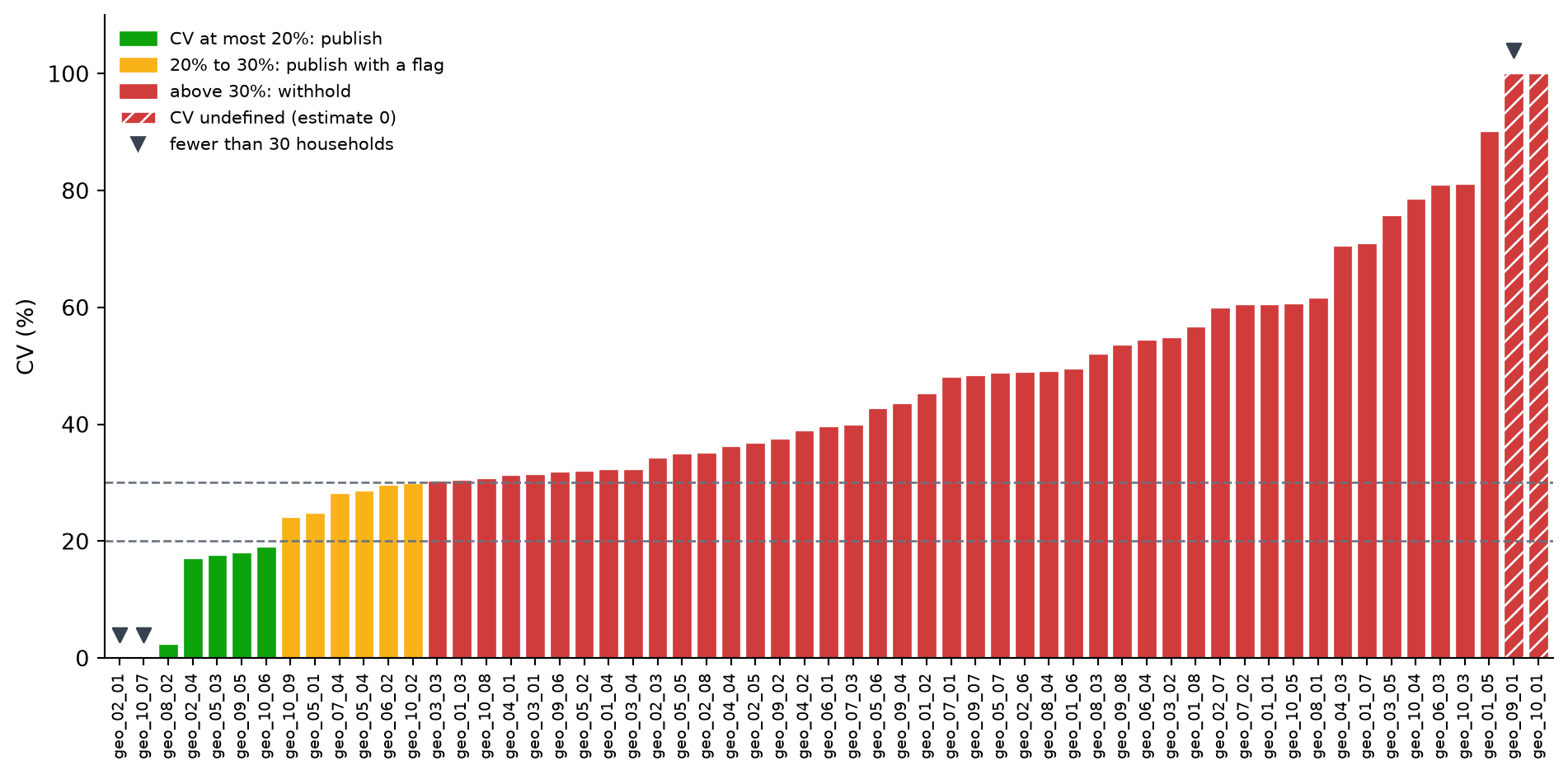
Most districts are red. Sample size does not explain it: across these districts, the number of households sampled and the CV are unrelated. The CV of a rate is larger when the rate is small, and sampling households in clusters (EAs) inflates it. The smallest CVs come from districts sampled in one to seven EAs, where the variance itself rests on very little: geo_08_02’s 2% rests on two EAs.
Count the districts in each band:
district.select(
    (pl.col("cv") <= 0.2).sum().alias("CV at most 20%"),
    ((pl.col("cv") > 0.2) & (pl.col("cv") <= 0.3)).sum().alias("20% to 30%"),
    (pl.col("cv") > 0.3).sum().alias("above 30%"),
    pl.col("cv").filter(pl.col("cv").is_finite()).median().alias("median CV"),
)
shape: (1, 4)
| CV at most 20% | 20% to 30% | above 30% | median CV |
|---|---|---|---|
| u32 | u32 | u32 | f64 |
| 7 | 6 | 46 | 0.389205 |
Four districts have a standard error of zero:
district.filter(pl.col("se") < 1e-6).select(
    "geo2", "est", "se", "cv", "n", "df"
)
shape: (4, 6)
| geo2 | est | se | cv | n | df |
|---|---|---|---|---|---|
| str | f64 | f64 | f64 | i64 | f64 |
| "geo_02_01" | 0.12 | 3.4694e-18 | 2.8912e-17 | 25 | 0.0 |
| "geo_09_01" | 0.0 | 0.0 | inf | 25 | 0.0 |
| "geo_10_01" | 0.0 | 0.0 | inf | 50 | 1.0 |
| "geo_10_07" | 0.44 | 9.3675e-17 | 2.1290e-16 | 25 | 0.0 |
geo_02_01andgeo_10_07were sampled in a single EA, a singleton PSU. The design gives no information on its variance (dfis 0), so the standard error and CV are zero up to rounding: these districts sit at the left of the chart, in green, without being precise. svy offers several ways to handle singletons (see Singleton PSUs); these tutorials leave them as they are.geo_09_01andgeo_10_01have no poor household in the sample. The estimate is 0, its standard error is 0, and the CV is undefined: the hatched bars at the right.
A minimum sample size
A CV is only as good as the variance behind it. A common rule of thumb therefore also withholds estimates based on fewer than about 30 sampled units, whatever their CV. Here it catches the three districts sampled in a single EA, marked with a triangle on the chart, including the two whose CV looks perfect. Apply both rules:
publishable = district.filter((pl.col("cv") <= 0.3) & (pl.col("n") >= 30))

print(f"Publishable districts: {publishable.height} of {all_districts.height}")
Publishable districts: 11 of 61Of the 61 districts, 11 pass both rules. The other 50 do not: 46 have a CV above 30%, including the 2 with no poor household; 2 are singletons; and 2 have no sample at all.
How far off are they?
Because the data are synthetic, the census also records every household’s expenditure, so the true poverty rate of each district is known:
truth = hld_census.group_by("geo2").agg(
    (pl.col("tot_exp") < pl.col("hhsize") * 1800).mean().alias("true_rate")
)

check = district.join(truth, on="geo2").with_columns(
    (pl.col("est") - pl.col("true_rate")).alias("error")
)

rmse_direct = check.select((pl.col("error") ** 2).mean().sqrt()).item()
print(f"Direct estimates, RMSE against the truth: {rmse_direct:.3f}")

check.select("geo2", "n", "est", "true_rate", "error").sort(
    pl.col("error").abs(), descending=True
).head()
Direct estimates, RMSE against the truth: 0.155
shape: (5, 5)
| geo2 | n | est | true_rate | error |
|---|---|---|---|---|
| str | i64 | f64 | f64 | f64 |
| "geo_02_01" | 25 | 0.12 | 0.572237 | -0.452237 |
| "geo_10_01" | 50 | 0.0 | 0.423086 | -0.423086 |
| "geo_09_01" | 25 | 0.0 | 0.412918 | -0.412918 |
| "geo_05_01" | 50 | 0.055238 | 0.432254 | -0.377016 |
| "geo_05_03" | 100 | 0.69343 | 0.367367 | 0.326063 |
Against an average poverty rate of about 0.23, an error of 0.155 is large, and the largest errors are in the districts with the fewest sampled households. The tutorials report the same RMSE for each model-based estimate.
WarningOnly with synthetic data
In practice the truth is unknown, which is why the model’s own measures of uncertainty (MSE and CV) matter. The comparison here shows what those measures cannot: how close the estimates actually are.
What the tutorials do
The survey alone cannot give publishable district estimates. The census can help: it records, for every household in every district, characteristics related to poverty, such as access to piped water, a flush toilet, or a mobile phone. A small area model links the survey to these covariates and uses the link to estimate each district, including the two the survey did not reach. Each estimate comes with its mean squared error (MSE), so its precision can be checked against the same publication rules.
svy-sae offers two families of models, and the tutorials apply both to these districts:
- Area-level models start from the district direct estimates above and district averages of the census covariates. They need only aggregates, which makes them the common choice when unit records cannot be shared.
- Unit-level models start from the household records of the survey and the census. They use more of the data and estimate any indicator of the distribution, such as the poverty gap.
Summary
This tutorial computed direct poverty rates with svy and measured them:
- National and regional estimates: precise, with CVs mostly below 25%
- District estimates: 59 of 61 districts sampled, 25 to 475 households each, a median CV of 39%
- Publication rules: with a 30% CV rule and at least 30 households, 11 of 61 districts could be published
- Accuracy: an RMSE of 0.155 against the true rates
- The way forward: models that combine the survey with census covariates
Next steps
Start with area-level models
Continue to Preparing area-level inputs →
References
World Bank. 2023a. “Synthetic Data for an Imaginary Country, Full Population, 2023.” World Bank, Development Data Group. https://doi.org/10.48529/78M1-AE09.
———. 2023b. “Synthetic Data for an Imaginary Country, Sample, 2023.” World Bank, Development Data Group. https://doi.org/10.48529/MC1F-QH23.